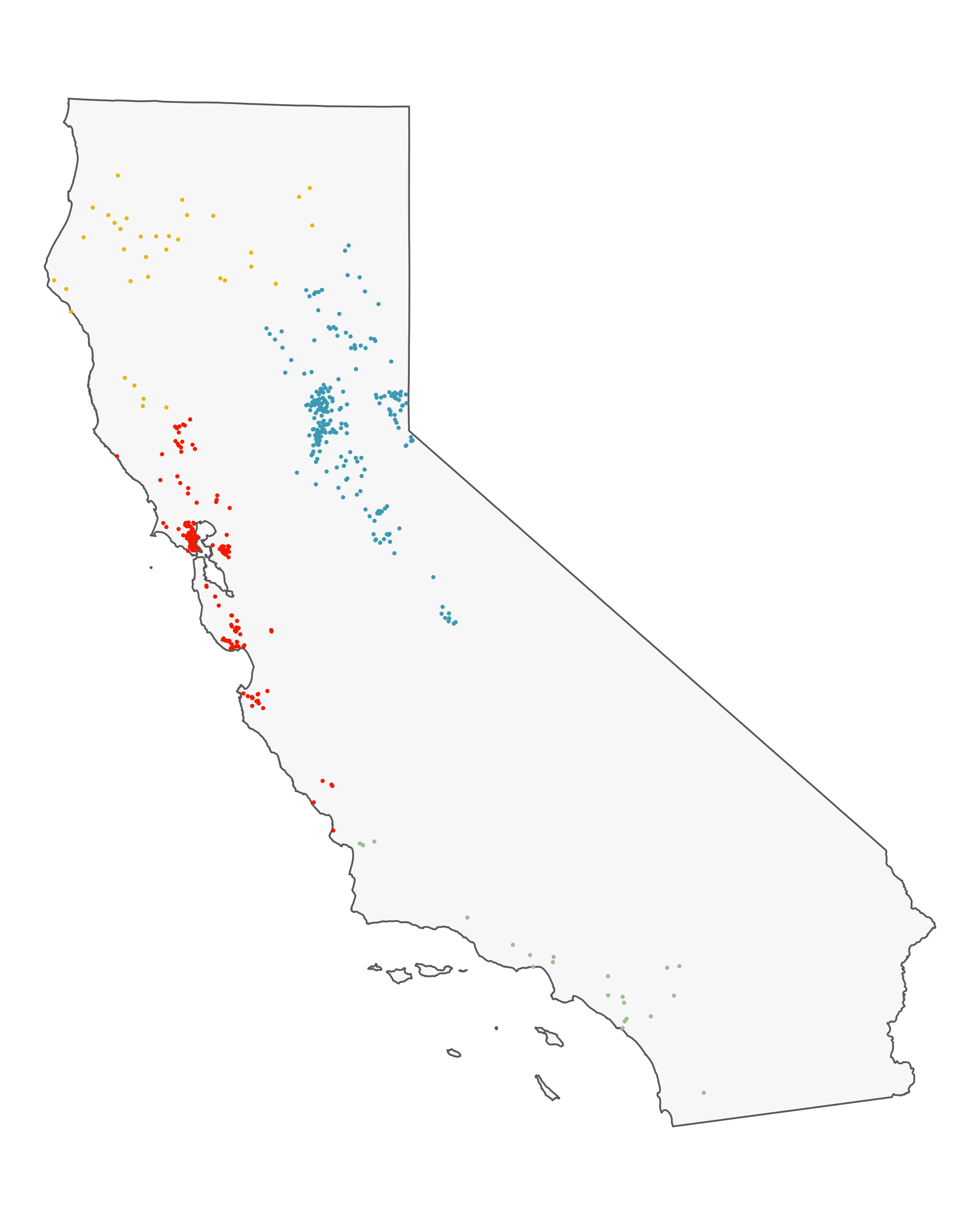
The Problem: I’ve got a list of lat-long coordinates for Firewise sites across California, and I want to understand, ata rudimentary level, where these sites fall in the grand scheme of Wildfire Hazard.

The sites are spread throughout California, and I have a suspicion there’s some regionality trends I might want to delve into later, so I do a some basic K-nearest neighbor clustering to split the sites into four distinct groups: Southern Cali (green), the Bary Area (red), Northern Cali (yellow), and the Sierras (blue).

Site Map of Firewise Sites (circa 2021)

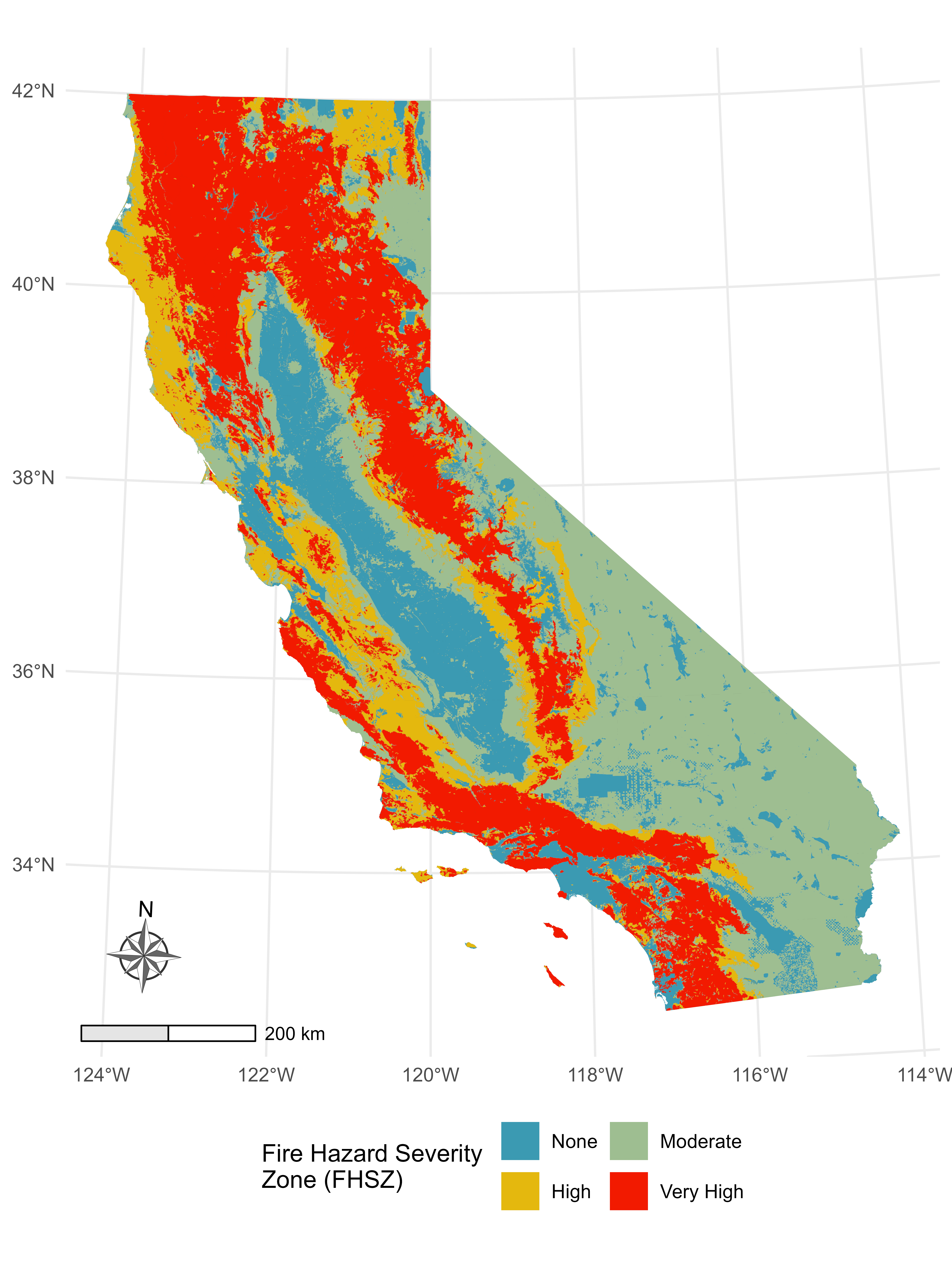
Then, I’ve got this underlying Fire Hazard Severity Map from CALFIRE.

Cal Fire's Fire Hazard Severity Zones

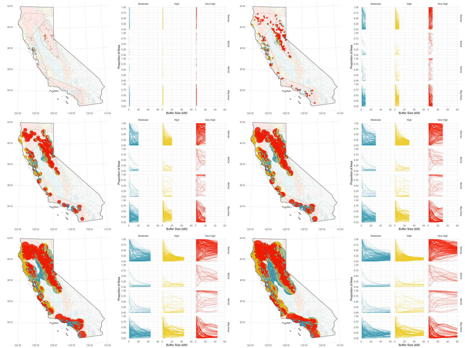
Rather than pick an arbitrary buffer size, like 5 Km or something subjective and prone to sensitivity issues (this is the big issue I have with buffer analyses), I decided to compute a continuous buffer from 1-60 Km to get a sense of how the fire hazard environment changes over distance.

Computing the Buffers

I understand why computing continuous buffers isn’t common, it can get pretty messy. I have 500 site points, and three FHSZ values (Moderate, High, Very High), and I want to calcultae the proportion of area each FHSZ occuppies throughout the continuous buffer (ie %Very High, %High, etc).

I thought this would be a good oportunity for parallel computing - its the same redundant calculation over and over again. So rather than just for-loop it (or apply it), I used the foreach package to parallelize a for-loop to calculate the percent area of each risk zone, for each buffer size from 1-60km.

Registering clusters for parallel computation

library(parallel)
library(doParallel)

cores <- detectCores()
cl <- makeCluster(cores[1]-1)
registerDoParallel(cl)

The Loop

mod <- list()
high <- list()
vhigh <- list()
all <- list()
cbuff <- foreach(i = 1:50) %dopar% {
  library(sf)
  buff        <- st_intersection(st_buffer(sites.sf[,1], i*1000), cali) 
  
  buff.area <- st_area(buff)
  mod[[i]]    <- st_intersection(risk[2,], buff)
  mod[[i]]$buff <- i*1000
  mod[[i]]$area <- as.numeric(st_area(mod[[i]]))
  mod[[i]] <- st_drop_geometry(mod[[i]])
  
  high[[i]]    <- st_intersection(risk[1,], buff)
  high[[i]]$buff <- i*1000
  high[[i]]$area <- as.numeric(st_area(high[[i]]))
  high[[i]] <- st_drop_geometry(high[[i]])

  vhigh[[i]]    <- st_intersection(risk[4,], buff)
  vhigh[[i]]$buff <- i*1000
  vhigh[[i]]$area <- as.numeric(st_area(vhigh[[i]]))
  vhigh[[i]] <- st_drop_geometry(vhigh[[i]])
  
  all[[i]] <- c(mod[i], high[i], vhigh[i])
  all
}

stopCluster(cl)
end <- proc.time()

ttime <- end - st

df.mod <- as.data.frame(do.call(rbind, mod))
df.high <- as.data.frame(do.call(rbind, high))
df.vhigh <- as.data.frame(do.call(rbind, vhigh))

df <- bind_rows(df.high, df.mod, df.vhigh)

lapply(list(df.mod, df.high, df.vhigh), function(x){rm(x)})

library(magick)
## list file names and read in
imgs <- list.files("plots/gif", full.names = TRUE)
img_list <- lapply(imgs, image_read)

## join the images together
img_joined <- image_join(img_list)

## animate at 2 frames per second
img_animated <- image_animate(img_joined, fps = 2)


## save to disk
image_write(image = img_animated,
            path = "plots/cont_buff2.gif")

Gif!!